Maximum Reach Estimates for Low-Voltage DC Power Delivery

Quote of the Day

Before you act, listen. Before you react, think. Before you spend, earn. Before you criticize, wait. Before you pray, forgive. Before you quit, try.

— Ernest Hemingway


Introduction

Figure 1: Wiring is Getting Out of Control and People are Trying to Use Existing Cables to Run Power. (Source)

Figure 1: Wiring is Getting Out of Control and People are Trying to Use Existing Cables to Run Power. (Source)

It is no secret that I prefer Mathcad for the vast bulk of my computational work, but I live in a world in which Excel is universally available. As such, I must prepare Excel workbooks for others to use. Today, I was asked to prepare an Excel worksheet that our salesman could use for estimating the maximum range over which different combinations of wire and voltage could deliver useful power. I include my Excel workbook here for those who wish to follow along.

I am facing quite a bit of DC analysis lately because customers are doing everything they can to reuse existing cabling. Many customers are facing wiring nightmares (Figure 1) and are trying to find ways of minimizing the clutter.

This analysis is just an exercise in applying Ohm's law, but it does illustrate a type of calculation that electrical engineers regularly encounter.

I actually performed the calculation in two different ways:

  • filled down formulas
  • data table

As you can see in my workbook, both methods give the same answer – as they should.

Background

Schematic

Figure 2 shows my schematic model of this DC powering configuration.  The key features of this schematic are:

  • The cable consists of pairs of wires.
  • The resistance of the each wire in the pair is identical.
  • The wire pairs will be connected in parallel, so the total cable resistance will be {{R}_{T}}=2\cdot \frac{{{{R}_{W}}}}{N}, where N is the number of wire pairs in parallel.
  • Each wire end is inserted into a connector, which will add a contact resistance (RC).
 Figure 2: Electrical Schematic.

Figure 2: Electrical Schematic.

Basic Formulas

Figure 3 shows the formulas used to determine the maximum cable reaches. While it looks complex, it is just Ohm's law being applied to the configuration of Figure 3.

Figure 3: Reach Formula Summary.

Figure 3: Reach Formula Summary.

Analysis

Parametric Assumptions

Figure 4 shows my parametric assumptions.

Figure M: Key Analysis Parameters.

Figure 4: Key Analysis Parameters.

Final Result

Figure 5 shows my final result. While this specific result is important for some staff members, my interest here is sharing how the calculations are performed using Excel (workbook).

Figure 4: Max Reach Table.

Figure 5: Max Reach Table.

Conclusion

This post was focused on how to present a simple electrical analysis in Excel. While Excel is not an ideal tool for mathematical work, I was able to prepare a workbook that others found useful and were able to modify to suite their needs.

Save

Save

Save

Posted in Electronics | 1 Comment

Bore Diameter Measurement Using Gage Balls

Quote of the Day

Cost is more important than quality, but quality is the best way to reduce cost.

Genichi Taguchi. I have much empirical evidence for the truth of his statement.


Introduction

Figure M: Hole Diameter Measurement Using Gage Balls Example.

Figure 1: Hole Diameter Measurement Using Gage Balls Example.

I am continuing to work through the metrology examples on this web page as part of junior machinist self-training. Today's technique shows how to use gage balls to measure the bore diameter of a cylinder (Figure 1). You can measure a bore diameter using a micrometer, but I have concerns that I might be measuring along a chord instead of a diameter – this error would result in too small of a result. The gage ball approach should eliminate that type of error.

In this post, I will work through the basic geometry associated with this measurement and will work an example.

Background

I have discussed gage balls in two previous blog posts (here and here), which should provide any background that you need.

Analysis

Derivation

Figure 2 shows how I defined my variables. The analysis involves solving the right triangle formed by X, Y, and the line formed by r1 and r2.

Figure 2: Definition of Terms.

Figure 2: Definition of Terms.

Figure 3 shows the algebra involved with the solving for the bore diameter (dB). Because I work in Mathcad, most the algebraic manipulations are hidden. If you desire, you can see the algebra worked out in my response to a question below the post.

Figure 2: Derivation of Bore Diameter Formula.

Figure 3: Derivation of Bore Diameter Formula.

Example

Figure 4 shows my results after applying the values in Figure 1 to the bore diameter formula. The result is very close to the bore diameter of 4.0000 on the scale drawing.

Figure 4: Formula Results for Conditions of Figure 1.

Figure 4: Formula Results for Conditions of Figure 1.

Conclusion

I am almost done reviewing the use of roller gages and gage balls. A couple more  examples will complete my set of canonical applications.

Save

Save

Save

Save

Save

Save

Save

Save

Save

Posted in Metrology | 5 Comments

Relationship Between Battery Cold Cranking Amps and Capacity

Quote of the Day

The difference between successful people and very successful people is that very successful people say 'no' to almost everything.

— Warren Buffet. Many people do not accomplish their goals because they spend the bulk of their time on items that really are just distractions. You need to look at your time usage, figure out which recurring items are taking time, yet providing little real value, and minimize them.


Introduction

Figure 1: Typical Flooded Cell Car Battery.

Figure 1: Typical Flooded Cell Car Battery. (Source)

Many battery manufacturers do not specify the Ampere-Hour (AH) ratings for their automotive products because Cold Cranking Amperes (CCA) are more important in automotive applications than AH ratings. Car applications tend to focus on the ability of the battery to crank the engine when both the battery and car are cold. While reading a post on an automotive forum about batteries, I saw the following statement made about the relationship between a battery's CCA and AH ratings.

I have read on the box of that Inox battery conditioner that for a battery over 600 CCA you simply multiply the CCA by .07 to give you the Amp Hours for that battery …

I have seen this statement before and did not believe it because batteries intended for capacity-dependent applications (e.g. backup power) are designed differently than batteries intended to deliver surge current (e.g. car batteries). I decided that it was time that I demonstrate that this relationship does not hold for specific batteries, but does have some merit for batteries in general.

Because France requires battery manufacturers post the AH specifications for all car batteries, I was able to find both CCA and AH specifications for a number of car batteries on European web sites. Once I gathered the data, I generated a graph that shows that there is not a general relationship between the CCA and AH. All you can say is that on average, increasing CCA ratings means increasing AH ratings. There is no simple relationship between AH and CCA that holds for all lead-acid automotive batteries.

All the analysis was done in Rstudio.

Background

Methodology

My approach was simple:

  • I randomly chose four car batteries from five different vendors.
  • I generated plots of AH versus CCA for each manufacturer.
  • I also generate a plot of AH versus CCA for all the batteries.

Data Set

Figure 2 show the set of battery data that I gathered. The batteries were randomly chosen from among the hundreds of choices.

Figure 2: List of Random Chosen Car Batteries.

Figure 2: List of Random Chosen Car Batteries.

Analysis

Figure 3 shows my graph of AH versus CCA for data of Figure 2. I also fitted lines to each of the vendors data. Note that there is a wide variation in how AH varies with CCA for each vendor. There is no formula that provides a good fit between AH and CCA for all automotive batteries. The fit is not even good for batteries from the same manufacturer. For a similar chart of batteries from a single manufacturer, see Appendix A.

Figure 3: Plot of Five Manufacturers, Four Batteries Each.

Figure 3: Plot of Five Manufacturers, Four Batteries Each. Note that I "jittered" the data so that points from different vendors would not sit on top of each other.

Figure 4 shows my overall curve fit. This line has a slope of 0.0688 AH/CCA, which agrees with the 0.07 AH/CCA statement on the Inox conditioner box. However, you can see that specific batteries are scattered far from the line.

Figure 4: Linear Curve Fit for All the Data.

Figure 4: Linear Curve Fit for All the Data.

For those who like to look at curve fit statistics, I also include Figure 5. The statistics shown are for lines that are function of CCA alone (Figure 4), and CCA and Brand (Figure 3).

For AH versus CCA line, we see that CCA is a very significant factor (red underline) but our R-squared value (fraction of variability explained) is only 50%. For the AH versus CCA and Brand line, we see that CCA is very significant and some Brands are significant,  but our R-squared value (fraction of variability explained) is only 85%.

Figure 5: Curve Fit Statistics.

Figure 5: Curve Fit Statistics.

Conclusion

While it might be tempting to estimate the AH rating of a battery from its CCA rating, there is not a simple relationship between these two battery parameters.

Appendix A: Yuasa Example

In Figure 6, Yuasa has published a graph similar to my Figure 3. Notice how the lines have roughly the same slopes, but different intercepts. As I always say, a battery is a nonlinear function of everything.

Figure 6: Battery CCA Versus Capacity. (Source)

Figure 6: Battery CCA Versus AH. (Source)

Save

Save

Save

Save

Save

Save

Save

Save

Save

Save

Save

Save

Save

Posted in Batteries | 20 Comments

Remote Car Starter Can Drain Car Battery Within a Week

Quote of the Day

If a free society cannot help the many who are poor, it cannot save the few who are rich.

- John F. Kennedy


Introduction

Figure 1: 2016 Honda CR-V.

Figure 1: 2016 Honda CR-V.

My Montana-based son mentioned that his wife's 2016 Honda CR-V (Figure 1) will not turn-over after sitting in the garage for five days. To be honest, there was a part of me that wasn't surprised in the slightest that the car wouldn't start. What do you expect to happen when it has been at a standstill for five days? The other side of me, though, thought that something more serious had to have been going on if something like this had happened in such a short amount of time. I'm just thankful that it was this problem we had to deal with and not something more severe. Imagine if she had found herself in a car accident because of underlying problems? It would be unthinkable, but I guess we should be lucky that my son's wife had taken the time to read something like this safeco insurance review when it came to renewing her insurance policy, so at least she would be covered if something else were to happen. Of course, the fact that it wouldn't turn-over is worrying in itself.

No starting problems had occurred prior to early November. Unfortunately, I have had my share of car electrical problems and some of these problems have been hard to find. However, this is a new car and under warranty, so I recommended that he just take it into the dealer. He took the car into the Honda dealer, who told him that this is the result of the current discharge imposed on his car battery by his aftermarket remote start system (with cell phone interface, sometimes called a drone), which was verified to be within specification –the car was operating normally.

In this post, I will discuss why this behavior is normal considering how the remote starter works and recent weather changes in Montana. I should mention that all modern cars will discharge their batteries over time because their computer systems are always on – their nominal current drain is about 30 mA. Even without a remote starter, the cars will discharge their batteries after about 3 weeks (Appendix A).

Background

Definitions

Cold Cranking Amps (CCA)
Cold cranking amperes (CCA) is the amount of current a battery can provide at 0 F (−18 C). (Source)
Parasitic Current Drain (iP)
Parasitic current drain can be defined as any electrical device that draws electric current when the ignition key is turned off. In the case of a remote starter, the radio receiver must be powered so that it can receive the starter signal. This receiver current draw is parasitic current drain. (Source)
Ampere-Hour (Ah) Capacity
An ampere hour or amp hour is a unit of electric charge, having dimensions of electric current times time, equal to the charge transferred by a steady current of one ampere flowing for one hour, or 3600 coulombs. Battery charge capacity is usually rated in Ah. (Source)

Battery Capacity Versus Temperature

Figure 2 shows the impact of temperature on the capacity of a lead-acid traction battery.

Figure 2: Traction Battery Capacity Versus Temperature.

Figure 2: Traction Battery Capacity Versus Temperature.

CCA Versus Battery Capacity

Figure 3 shows that a battery's available Cold Cranking Amperage (CCA) decreases with reduced battery capacity. For the analysis of this post, I will assume that a battery's available CCA reduces proportionately with its capacity. Figure 3 originally came from a Yuasa technical specification.

Figure M: Battery CCA Versus Capacity. (Source)

Figure 3: Battery CCA Versus Capacity. (Source)

Cranking Current Required By a Car Versus Temperature

Figure 4 shows that the battery's available CCA decreases with lower temperature as the car's need for cranking amperage increases. I refer to this situation as "bad squared".

Figure 4: Car Cranking Amperage Required Versus Temperature. (Source)

Figure 4: Required Car Cranking Amperage Versus Temperature. (Continental Battery)

Problem Statement

Here is what I was able to find out about my son's situation:

  • His remote starter is rated to have a maximum parasitic current draw of 75 mA.
  • The measured remote starter parasitic current drain is 70 mA – it is within specification for remote starter units with a cell-phone interface. Other folks report similar parasitic loads.
  • Separate from the cell phone-based car starter parasitic current drain, the car itself has a parasitic current drain of 30 mA to support its onboard computer. This means that the total expected parasitic drain is ~100 mA = 70 mA + 30 mA, which is in rough agreement with reports on other web sites.
  • The car battery experiences the parasitic current drain for 5 days.
  • His wife just had a baby and is on maternity leave. The car had been driven every day prior to October 30th. After October 30th, the car has been driven sporadically.
  • The car is only driven short distances. I am guessing that the battery is never fully charge because of how it is started, driven a short distance and stopped. I will assume the battery routinely sits at 75% charge during normal use. In fact, cars brought in for service typically have batteries with 70% of a full charge.
  • The weather recently turned cold. The temperature had been in the 70 F (~25 C) range and now is about 18 F (-8 C) in the morning when the car is being started. This temperature drop reduces the battery capacity to 60% of its charge at the specification temperature (77 F).
  • I will assume that the effective CCA rating is proportional to the Ah rating, which is illustrated in Figure 3.
  • The car battery is rated for 500 CCA. I do not have a specification for its ampere-hour capacity, which is important when determining capacity. Batteries of similar size and CCA ratings have a capacity rating of 50 Ah.

This is enough information for me to figure out what is going on.

Analysis

Figure 5 shows my analysis of the battery capacity. What I calculated is that the battery's capacity has reduced by ~75%. This results in a large decrease in the cranking amps available (justification in a later post) and results in slow or no cranking when attempting to start the car.

Figure 5: Battery Capacity Analysis

Figure 5: Battery Capacity Analysis

Conclusion

I am afraid that an additional parasitic battery load of 70 mA is enough to drain the battery sufficiently after five days to make starting difficult or impossible. This reminds me of a battery problem I had in my youth where a glove compartment light did not turn off and would slowly drain my battery. I could fix the light problem, but the remote starter must draw current to detect the radio start signal.

Appendix A: Computer Parasitic Leakage Example

Figure 6 shows a manual excerpt that illustrates how modern cars have computers that constantly drain charge from their batteries.

Figure 6: Chrysler 200 Manual Calling Out Battery Discharge.

Figure 6: Chrysler 200 Manual Calling Out Battery Discharge.

Posted in Batteries | 25 Comments

Angle Measurement Using Roller Gages

Quote of the Day

It is a universal truth that the loss of liberty at home is to be charged to the provisions against danger, real or pretended, from abroad.

— James Madison


Introduction

Figure 1: Angle Measurement Example.

Figure 1: Angle Measurement Example.

I am continuing to work through some basic metrology examples – today's example uses roller gages to measure the angle of a drilled hole (Figure 1). The technique discussed here uses two roller gages and a plug. The plug must fit the hole snugly (i.e. no backlash) as it will provide the surface that we will be measuring.  Using this approach assumes that you need a very accurate measurement of a hole's angle as rough measurements can be made using a protractor.

Background

This example is based on the material found on this web page. I will derive the angle relationship presented there (Equation 1) and present a worked example that is confirmed using a scale drawing (Figure 1).

Eq. 1 \displaystyle \theta \left( {{{L}_{1}},{{L}_{2}},{{D}_{1}},{{D}_{2}}} \right)=2\cdot \text{arctan}\left( {\frac{1}{2}\cdot \frac{{{{D}_{1}}-{{D}_{2}}}}{{{{L}_{1}}-\frac{{{{D}_{1}}}}{2}-\left( {{{L}_{2}}-\frac{{{{D}_{2}}}}{2}} \right)}}} \right)

where

  • L1 is the distance from reference to outside edge of roller gage.
  • L2 distance from reference to outside edge of roller gage.
  • D1 diameter of the first roller gage.
  • D2 diameter of the second roller gage.
  • θ is the angle of the drill hole relative to the surface that is drilled.

These variables are all indicated in Figure 2.

Figure 2: Reference Drawing Showing Critical Variables.

Figure 2: Reference Drawing Showing Critical Variables.

Analysis

Derivation

Figure 3 shows how to derive Equation 1. The basic derivation process is simple:

  • The center of each roller gage is on a line that is makes an angle of θ/2 with the plug.
  • The slope of line connecting the roller gage centers has the value tan(θ/2).
  • The line's slope is computed using the rise (\frac{{{{D}_{1}}}}{2}\cdot \left( {1+\tan \left( {\frac{\theta }{2}} \right)} \right)-\frac{{{{D}_{2}}}}{2}\cdot \left( {1+\tan \left( {\frac{\theta }{2}} \right)} \right)) and run (L1L2) values shown in Figure 2.
Figure 3: Derivation of Angle Relationship.

Figure 3: Derivation of Angle Relationship.

Example

Figure 4 shows works through the angle calculation example of Figure 1.

Figure 4: Worked Example Using Values From Figure 1.

Figure 4: Worked Example Using Values From Figure 1.

Conclusion

I have some designs I plan to build that have angled holes. This procedure will give me a way to accurately measure the angle of these holes.

Save

Save

Save

Save

Save

Save

Save

Save

Save

Save

Save

Save

Save

Save

Posted in Metrology | 2 Comments

Ensuring Stable DC Power Delivery To Switching Loads

Quote of the Day

Life is never made unbearable by circumstances, but only by lack of meaning and purpose.

Viktor E. Frankl


Introduction

Figure 1: Commercial LED Lightning Deployment Using DC Power Distribution.

Figure 1: Commercial LED Lightning Deployment Using DC Power Distribution. (Source)

I presented a seminar over lunch today on short-range DC power distribution, which I believe is one of the most exciting areas in electronics today.  AC power distribution has dominated power engineering since the "War of the Currents" ended with Westinghouse's AC system winning a decisive victory over Edison's DC system back in the 1890s. Starting in 1930s Europe, high-voltage DC distribution has slowly gained a foothold in some long-haul, high power distribution applications, but most power distribution has continued to be dominated by AC.

We are now seeing a resurgence in low-voltage DC power for use in short-range power distribution because of recent technology changes:

  • Increasing use of photovoltaics, which produce DC.
  • Increasing use of LED lighting, which can be powered more efficiently by DC.
  • Desire to use network cable to distribute both power and data (e.g. PoE).
  • Desire to reduce installation costs by eliminating the expense associated with ensuring that AC wiring is safe (e.g. conduit, heavy gauge wire, labor using highly-trained electricians, etc).

One issue that needs to be addressed is how to ensure the stability of a DC distribution when it is driving loads composed switching power supplies, which have a rather complicated input impedance function. One common approach is to apply the Middlebrook stability criterion, which provides a sufficient condition for a stable DC network. In this blog post, I will be discussing the derivation and application of the Middlebrook stability criterion.

My raw Mathcad file is included here (with PDF) if you wish to work through the examples yourself.

Background

History

RD Middlebrook published his criterion in the journal article "Input Filter Considerations, in Design and Application of Switching Regulators",  IEEE Industry Applications Society Annual Meeting, October, 1976. The Middlebrook criterion is commonly used because it is simple to apply, however it has relatively high implementation cost. For a discussion of the alternatives, see this presentation.

The Middlebrook criterion is also known as an impedance ratio criterion. I will demonstrate why it is called an impedance ratio criterion in Figure 5.

Middlebrook Criterion Statement

The following discussion summarizes a longer paper that I include here.

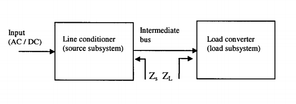
Figure 3 shows how power engineers usually define the source and input impedances of a power system.

Figure M: Simple Power System Model.

Figure 3: Simple Power System Model.

Using the impedance definitions illustrated in Figure 3, I usually see the Middlebrook criterion stated as follows:

A system will be locally stable if the magnitude of the input impedance of the load subsystem is larger than the magnitude of the output impedance of source subsystem.

You also often see engineers refer to the criterion's equivalent graphical form:

If the magnitude plots of the source (ZS) and load impedances  (ZL) do not intersect, the system is stable. If the impedance intersection occurs, the system may not be stable. If the impedance magnitude intersection occurs, the system will still be stable providing that the impedance ratio transfer function ZS/ZL satisfies the Nyquist stability test.

Figure 4 shows what a graphical analysis looks like (Source). The yellow cross-hatched region show that there is a potential stability problem with this system. Because the Middlebrook criterion is a sufficient but not necessary condition, more analysis is needed to determine if there is a real problem. In practice, most engineers would not do further analysis but instead would add some form of compensation network to eliminate the yellow cross-hatched region.

Figure 4: Graphical Analysis Example.

Figure 4: Graphical Analysis Example.

One advantage of the graphical approach is that it can be applied to measured impedance data. See Appendix A for an plot of an actual power supply input impedance. The measured data can be quite complex.

Analysis

Derivation

Figure 5 shows my pictorial view on how to "prove" the Middlebrook criterion. The process is straightforward:

  • Generate a model of the power converter output and the load.

    This step defines the critical impedance values (Zo1 and Yi2=1/Zi2) that are used to evaluate the stability of a power distribution system.

  • Perform a simple circuit analysis that yields two equations.
  • These equations can be represented as a control system graph.

    This step defines allows us to apply an existing stability criterion to this specific case.

  • This control system graph meets the requirements of the Small Signal Theorem, which provides the stability criterion.

    The Small Signal Theorem provides us a sufficient condition for stability, i.e. the system is stable if \left\| {{{Z}_{{o1}}}\left( {j\cdot \omega } \right)} \right\|\cdot \left\| {{{Y}_{{i2}}}\left( {j\cdot \omega } \right)} \right\|<1 . This is the key result.

  • Express Yi2 as 1/Zi2, which gives us the impedance ratio criterion, i.e. \frac{{\left\| {{{Z}_{{o1}}}\left( {j\cdot \omega } \right)} \right\|}}{{\left\| {{{Z}_{{i2}}}\left( {j\cdot \omega } \right)} \right\|}}< 1.
Figure 5: Illustration Outlining the Proof of the Middlebrook Stability Theorem.

Figure 5: Illustration Outlining the Proof of the Middlebrook Stability Theorem.

Worked Example: Uncompensated Case

I found a good paper that illustrated how to apply Middlebrook criterion in practice, and I will work through this paper in detail here.

Figure 6 shows a typical power supply situation and the sufficient conditions for stability in this case (light yellow highlight). This configuration may not be stable, but can often be made stable by adding a lossy capacitor, which I discuss in the following section.

Figure 5: Typical Power Supply Situation with No Compensation.

Figure 6: Typical Power Supply Situation with No Compensation.

Worked Example: Lossy Capacitor Compensation

Figure 7 shows how adding a lossy capacitor may stabilize the circuit of Figure 6. The analysis shown in Figure 7 is for a simplified version of Figure 6 – the algebra quickly gets out of control otherwise.

Figure 6: Effect of Lossy Input Capacitor.

Figure 7: Effect of Lossy Input Capacitor on Stability for the Circuit of Figure 6.

Conclusion

I have used the Middlebrook stability criterion for years, but have never taken the time to write down a tutorial for my staff. My recent seminar preparation provided me an excuse to finally write down a tutorial.

Appendix A: Measured Power Supply Input Impedance

Figure 7 shows a graph of an actual power supply input impedance (Source).

actual

Posted in Electronics, Power Over Ethernet | Comments Off on Ensuring Stable DC Power Delivery To Switching Loads

Radius Measurement Using Roller Gages

Quote of the Day

There are no secrets to success. It is the result of preparation, hard work and learning from failure.

— Colin Powell, general and statesman.


Introduction

Figure 1: Radius Measurement Using Two Gage Rollers and a Surface Plate.

Figure 1: Radius Measurement Example Using Two Gage Rollers and a Surface Plate.

This post will demonstrate how to measure the radius of an arc using two roller gages.  While I am a very amateur machinist, I have on occasion needed to measure the radius of an arc (i.e. partial circle) and have not been sure how to approach that measurement. It turns out to be simple given two equal diameter roller gages and a surface plate. You can determine by taking one measurement and knowing the roller gage diameter.

Background

I have been reading this web page on metrology, and this post consists of my notes from reading this web page. The key formula for measuring the radius of curvature for an arc is given by Equation 1.

Eq. 1 \displaystyle R=\frac{{{{{\left( {L-d} \right)}}^{2}}}}{{8\cdot d}}

where (referring to Figure 2).

  • R is the radius of the arc we want to measure.
  • d is the diameter of the two roller gages – they must be equal diameter.
  • L is the distance between the two roller gages as measured from their points of maximum separation.

Analysis

Derivation Geometry

The geometric situation is simple and illustrated in Figure 2. The radius of the yellow circle (R) is what needs to be measured. Note that we do not need a full-circle to apply this method – we can work with an arc. The only direct measurement I need to make is of L.

Figure 2: Radius Measurement Using Gage Balls Scenario.

Figure 2: Radius Measurement Using Gage Rollers Scenario.

Derivation and Example

Figure 3 shows the derivation, which consists of applying the Pythagorean theorem and simplifying. I also include my calculations for the example of Figure 1. The mathematical result equaled the value on my scale drawing (Figure 1).

Figure 3: Formula 1 Proof and Worked Example Using Figure 1

Figure 3: Proof and Worked Example Using the configuration in Figure 1.

Conclusion

I have struggled to measure the radii of various partially circular objects like bowls. Using a couple of roller gages gives me a simple way to measure the radius of curvature for these partial circles.

Save

Save

Save

Save

Save

Save

Save

Save

Posted in Construction, Geometry, Metrology | 3 Comments

Ion Propulsion Math

Quote of the Day

Telling a story is one of the best ways we have of coming up with new ideas, and also of learning about each other and our world.

Richard Branson


Introduction

Figure 1: Dawn Mission Profile. (Source)

Figure 1: Dawn Mission Profile. (Source)

NASA has a project known as Dawn that put a space probe in orbit around the asteroids Vesta and then CeresCSPAN presented an excellent Dawn mission briefing given by Marc Rayman, the Mission Director and Chief Engineer.  One of the most interesting aspects of the  Dawn spacecraft is its use of an ion thruster to maneuver it from one destination to another. This post presents some simple math that can be used to determine some of its key performance characteristics.

This briefing was for the general public and presented some excellent material. For those who like to look at my raw files, I include my Mathcad, PDF, and XPS versions here.

Background

Dawn Spacecraft Information

The following quote from the Wikipedia article on the Dawn spacecraft provides lots of data for me to use in my analysis.

The Dawn spacecraft is propelled by three xenon ion thrusters … and uses only one at a time. They have a specific impulse of 3,100 s and produce a thrust of 90 mN. The whole spacecraft, including the ion propulsion thrusters, is powered by a 10 kW (at 1 AU) triple-junction gallium arsenide photovoltaic solar array manufactured by Dutch Space. Dawn was allocated 275 kg (606 lb) of xenon for its Vesta approach, and carried another 110 kg (243 lb) to reach Ceres, out of a total capacity of 425 kg (937 lb) of on-board propellant. With the propellant it carries, Dawn can perform a velocity change of more than 10 km/s over the course of its mission, far more than any previous spacecraft achieved with onboard propellant after separation from its launch rocket.

I can summarize this data with the following list:

  • The thruster provides a thrust of 90 mN
  • The thruster generates a specific impulse of 3,100 s.
  • The thruster and fuel supply can provide a total velocity change ΔV= 10 km/s.
  • The photovoltaic array has a maximum power output of 10 kW @ 1 AU.
  • fuel mass of 425 kg.

I also found some additional information useful:

  •  xenon molecules at a velocity of 30 km/s. (Source)
  • maximum ion thruster input power level of 2.3 kW. (Source)
  • ion thruster power efficiency of 61%. (Source)
  • Dawn spacecraft Beginning of Life (BOL) mass of 1240 kg. (Source)

Dawn Thruster Block Diagram

Figure 2 shows a block diagram of Dawn's ion thruster. The basic construction is  reminiscent of the electron gun in an old tube-type television.

The thruster concept is simple:

  • supply xenon from the propellant supply bottle to the ionization chamber
  • ionize the xenon
  • accelerate the xenon ions using a high-voltage electric field
Figure 2: Dawn Thruster Block Diagram. (Source)

Figure 2: Dawn Thruster Block Diagram. (Source)

Analysis

Objective

My plan is to compute the following spacecraft characteristics:

  • thrust (FIon)
  • fuel burn rate (m')
  • mission time (TMission)
  • ΔV

based on the

  • array power (P)
  • xenon molecular velocity (v)
  • fuel quantity (MFuel)
  • spacecraft mass (MBOL)
  • engine efficiency (η).

Solution Setup

Figure 3 shows how I setup this calculation.

Figure M: Analysis Setup.

Figure 3: Analysis Setup.

Ion engine molecular velocity

Determine Key Performance Indices

Figure 4 shows how I used the conservation of energy to derive formulas for the thrust and fuel burn rate. The analysis approach is simple:

  • Solar power (minus efficiency losses) is converted from photon energy to xenon ion energy.
  • The kinetic energy of the xenon ions is converted to a velocity.
  • The velocity and mass loss rate is then converted to a change in momentum.
  • The change in momentum is equivalent to force.

All the numbers obtained using this approach reasonably match the values quoted in the Wikipedia. I should note that the rated mission lifetime is 50K hours, but there is only enough fuel for 40K hours at full power (i.e. 1 AU from the Sun). The 40K hours is actually reasonable because the Dawn spacecraft will spend a significant amount of time in orbit about these Vesta and Ceres, so it will not have the thruster on all the time.

Figure 4 Mathcad Note: You will see that many of the variables in Figure 4's derivation are teal-colored rather than black-colored. For derivations, I often use a different variable style to prevent an early numeric definition from interfering with a downstream symbolic derivation. A different variable style in Mathcad means that a variable with the same name as a another style is treated as a different variable. Otherwise, Mathcad will substitute the upstream numeric value of the variable, which I do not want when I need a symbolic result.

Figure 4: Determination of Four Key Engine Parameters.

Figure 4: Determination of Four Key Engine Parameters.

Dawn Ion Thrust Dawn Fuel Burn Rate Dawn Mission Duration Dawn Delta V

Conclusion

I was able to use some simple math and physics to reproduce some of the key performance metrics for the Dawn spacecraft. This helps me understand how ion propulsion works and where it would be useful to use. Because it requires so much power, I can see where it would primarily be useful for spacecraft that are close enough to the Sun to use solar power. A radioactive battery (often used on deep space probes) would not provide sufficient power to make an ion drive work – Rayman makes this comment in his briefing.

The Dawn mission was very interesting. I want to commend Marc Rayman for the excellent briefings he has presented throughout the project. I have enjoyed keeping up with their discoveries about Vesta and Ceres.

Posted in Astronomy | 4 Comments

Homemade Roof Pitch Protractor

Quote of the Day

I like opera, I just don't want to be around the people who like opera.

Justice Clarence Thomas, during a discussion of Justice Scalia and Scalia's love of opera. During a working stint in Keyport, WA, I had a coworker who LOVED opera. Thus, I completely understand this statement.


Figure 1: Homemade Roof Protractor. (Source)

Figure 1: Homemade Roof Protractor. (Source)

As an amateur carpenter, I am always looking for simple and cheap construction tools. Recently, I have been working on improving my roof framing knowledge. During my reading on this topic, I saw this roof pitch protractor in a Journal of Light Construction (JLC) article . Notice how the template has a handle to make hauling it up a ladder easier. To get an accurate roof pitch, all you need to do is (1) place the template on the roof, (2) clamp a spirit level onto the template in the level position, and (3) read the pitch off the scale – simple, fast, accurate.

Save

Save

Save

Save

Posted in Construction | Comments Off on Homemade Roof Pitch Protractor

WW2 Casualty Rates By Country

Quote of the Day

Mistakes should be examined, learned from, and discarded; not dwelt upon and stored.

— Tim Fargo. I know a number of people that live their lives in constant fear of making mistakes. No one likes mistakes, but people who make no mistakes do not make anything. You must develop a work style that is tolerant of mistakes and that allows you to make them early when they are generally less costly.


Figure 1: WW2 Casualty Percentages By Country.

Figure 1: WW2 Casualty Percentages By Country. (Source)

I recently was watching a documentary on WW2 that mentioned that Greece and Yugoslavia suffered some of highest casualty rates during WW2. While I have read much about WW2, I had not looked at the casualty rates as a percentage of each country's population. I did some quick web searching and found that the Wikipedia has an excellent table summarizing WW2 casualties by country and population, which I imported into Excel and sorted by casualty rates. These percentages are mind numbing. While Greece and Yugoslavia suffered terribly, other countries suffered even more.

National traumas like WW2 last many generations. Over 150 years ago, we suffered a 2% loss of population during the Civil War, and that loss affects us to this day. One personal story will illustrate my point. I used to work in Panama City, Florida – a great place to be during the winter. Because of my accent, people knew I was not a local, and one coworker told me he would not hold the "Recent Unpleasantness" against me. I had to ask "What was the Recent Unpleasantness?" and was floored to find out it was the Civil War.

There are a couple of items in Figure 1 that I would like to highlight:

  • Nauru and Portuguese Timor
    Their occupation by the Japanese was particularly brutal.
  • Ruanda-Urundi
    While WW2 in Northern Africa is well documented, I had no idea of the casualties caused by WW2's demand for resources.

For those who wish to work with the data themselves, I include my Excel Workbook here.

Save

Save

Save

Save

Posted in History Through Spreadsheets, Military History | Comments Off on WW2 Casualty Rates By Country